Tracing for GGE

Some mixtures have a high-pressure equilibrium sometimes referred to as gas-gas equilibrium which is not connected to the low-temperature VLE curves. To get these isotherms, they can be constructed by the following recipe:

1. Trace a low-temperature isotherm where the phase envelope is open

2. Interpolate that low-temperature isotherm to get guess values for the concentrations and temperature for a given pressure

3. Trace the high-pressure isobar

4. Interpolate within the high-pressure isobar to find the molar concentrations matching the given temperature (corresponding to the high-pressure GGE)

5. Trace the isotherm starting at the GGE solution.

The datafiles in the HENEAR folder are from the supplemental information of the paper “Equations of State for the Thermodynamic Properties of Binary Mixtures for Helium-4, Neon, and Argon”, by Tkaczuk, Bell, Lemmon, Luchier, and Millet. https://doi.org/10.1063/1.5142275 . The HASH were added to the provided JSON format EOS

import teqp, numpy as np, pandas, matplotlib.pyplot as plt, scipy

BIP, DEP = teqp.convert_HMXBNC('HENEAR/HMX.BNC')
jconverted = {
    "kind": "multifluid",
    "model": {
        'components': ['HENEAR/Helium.json', 'HENEAR/Argon.json'], # already in CoolProp format
        "BIP": BIP,
        "departure": DEP
    }
}
model = teqp.make_model(jconverted)
ancHe = model.build_ancillaries(0)
ancAr = model.build_ancillaries(1)
T = 200.0 # K
rho = 1e4 # mol/m^3
z0 = 0.5
z = np.array([z0, 1-z0])
R = model.get_R(z)

# display(model.get_BIP(0,1,"F"))
# display(model.get_rhor(z), model.get_Tr(z))

# Check that the validation point from the paper is obtained
p_calc = T*rho*R*(1+model.get_Ar01(T, rho, z))
p_expected = 17128034.388362616 # Pa
assert(abs(p_calc/p_expected-1) < 1e-10)

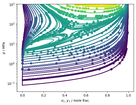
df = pandas.read_csv('HENEAR/HEAR_VLE.CSV')
sc = plt.scatter(df['x_He'], df['p/MPa'], c=df['T/K'])
sc = plt.scatter(df['y_He'], df['p/MPa'], c=df['T/K'])

def get_isoT(T):
    """ Get the "normal" isotherm for the binary mixture """
    # Densities from the normal ancillary equations
    rhoL0, rhoV0 = ancAr.rhoL(T), ancAr.rhoV(T) # start off at pure of the first component
    # Now we do a VLE calculation
    rhoL0, rhoV0 = model.pure_VLE_T(T, rhoL0, rhoV0, 10, molefrac = np.array([0,1]))
    # Trace the isothermal VLE
    j = model.trace_VLE_isotherm_binary(T, np.array([0, rhoL0]), np.array([0, rhoV0]))
    df = pandas.DataFrame(j) # Now as a data frame
    return df

def get_GGE_isobar(*, Tlow_K, p_MPa):
    dfisoT = get_isoT(Tlow_K)

    # Interpolate within the low temperature isotherm to get the molar concentrations at the given pressure
    t = scipy.interpolate.interp1d(dfisoT['pL / Pa'], dfisoT['t'])(p_MPa*1e6)
    RHOL = np.array(dfisoT['rhoL / mol/m^3'].tolist())
    RHOV = np.array(dfisoT['rhoV / mol/m^3'].tolist())

    rhoL0 = scipy.interpolate.interp1d(dfisoT['t'], RHOL[:,0])(t)
    rhoL1 = scipy.interpolate.interp1d(dfisoT['t'], RHOL[:,1])(t)
    rhoV0 = scipy.interpolate.interp1d(dfisoT['t'], RHOV[:,0])(t)
    rhoV1 = scipy.interpolate.interp1d(dfisoT['t'], RHOV[:,1])(t)

    rhovecL0 = np.array([rhoL0, rhoL1])
    rhovecV0 = np.array([rhoV0, rhoV1])
    dfisop = pandas.DataFrame(model.trace_VLE_isobar_binary(p=p_MPa*1e6, T0=Tlow_K, rhovecL0=rhovecL0, rhovecV0=rhovecV0))
    return dfisop

Tlow_K = 75 # K
GGE_1GPa = get_GGE_isobar(Tlow_K=Tlow_K, p_MPa=1000)

def get_GGE_isoT(T_K, init_c=1.0):
    """ Get the "GGE" isotherm for the binary mixture """

    # Interpolate within the high pressure isobar to get the molar concentrations at the given pressure
    t = scipy.interpolate.interp1d(GGE_1GPa['T / K'], GGE_1GPa['t'])(T_K)
    RHOL = np.array(GGE_1GPa['rhoL / mol/m^3'].tolist())
    RHOV = np.array(GGE_1GPa['rhoV / mol/m^3'].tolist())

    rhoL0 = scipy.interpolate.interp1d(GGE_1GPa['t'], RHOL[:,0])(t)
    rhoL1 = scipy.interpolate.interp1d(GGE_1GPa['t'], RHOL[:,1])(t)
    rhoV0 = scipy.interpolate.interp1d(GGE_1GPa['t'], RHOV[:,0])(t)
    rhoV1 = scipy.interpolate.interp1d(GGE_1GPa['t'], RHOV[:,1])(t)

    rhovecL0 = np.array([rhoL0, rhoL1])
    rhovecV0 = np.array([rhoV0, rhoV1])
    x0 = rhovecL0[0]/sum(rhovecL0)
    xspec = np.array([x0, 1-x0])
    code, rhovecL0, rhovecV0 = model.mix_VLE_Tx(T, rhovecL0, rhovecV0, xspec, 1e-12, 1e-12, 1e-12, 1e-12, 30)

    # Trace the isothermal VLE
    opt = teqp.TVLEOptions(); opt.calc_criticality = True; opt.init_c = init_c
    return pandas.DataFrame(model.trace_VLE_isotherm_binary(T, rhovecL0, rhovecV0, opt))

for T in df['T/K']:
    # Normal VLE traces starting at the pure fluid (easy part)
    try:
        # Build & plot the isotherm
        df = get_isoT(T)
        plt.plot(df['xL_0 / mole frac.'], df['pL / Pa']/1e6, c=sc.to_rgba(T))
        plt.plot(df['xV_0 / mole frac.'], df['pL / Pa']/1e6, c=sc.to_rgba(T))
    except: pass

    # Now we try to initiate a trace starting from the 1 GPa isobar, at the given
    # temperature
    for init_c in [-1, 1]:
        try:
            df2 = get_GGE_isoT(T_K=T, init_c=init_c)
            plt.plot(df2['xL_0 / mole frac.'], df2['pL / Pa']/1e6, c=sc.to_rgba(T))
            plt.plot(df2['xV_0 / mole frac.'], df2['pL / Pa']/1e6, c=sc.to_rgba(T))
        except: pass

plt.gca().set(xlabel='$x_1$, $y_1$ / mole frac.', ylabel='p / MPa')
plt.yscale('log')
plt.ylim(None, 1e3)
plt.show()